
A powerful feature of Microsoft Excel that I encourage everyone to check out is the Pivot Table. This element of Excel allows you to get great insights into your data.
One thing that confuses people though is when they add to their source data but the Pivot Table does not reflect the changes.
Creating a Dynamic Pivot Table
The trick is to create a “dynamic named range”. Rather than just add your table in the usual way, you need to create your pivot table using the named range, then you can add data, refresh, and the new data will automatically show up.
Creating the Named Range
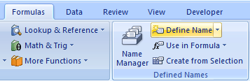
To create your named range in Excel 2007 go to Formulas > Define Name
In the Refers To box, enter an Offset formula. This defines the range size in the following way:
=OFFSET(Data!$A$1,0,0,COUNTA(Data!$A:$A),7)
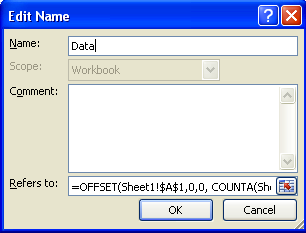
- Reference cell: Data!$A$1
- Rows to offset: 0
- Columns to offset: 0
- Number of Rows: COUNTA(Data!$A:$A)
- Number of Columns: 4
Create the Pivot Table using Your Named Range
Now you need to create the pivot:
-
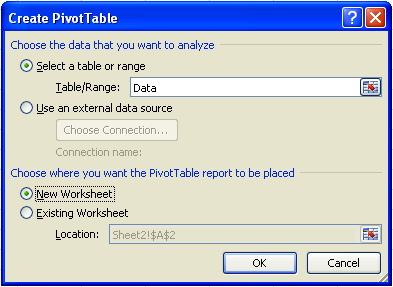
- Choose Insert > PivotTable
- Choose Insert > PivotTable
-
- Select Table/Range
- For the range, type your range name, e.g. Data
- Click OK
- Continue creating the pivot table as you normally would …
/ 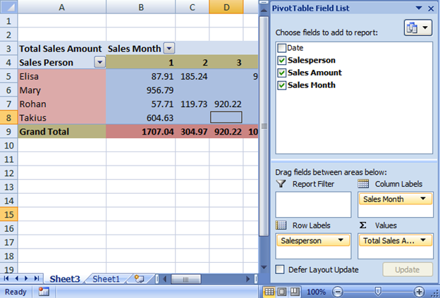
- Click OK
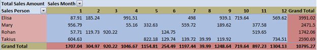
And there you have it – Your dynamic pivot table.
Summary
As is usual with the more powerful Excel features, knowing the trick is just half the battle. Then you need to put the knowledge into practice! Why not create some test pivot tables now so you can really get to grips with this great functionality?
P.S.
Don’t forget to check out our PDF to Excel Converter. It can save you a lot of precious time and improve your productivity.