Cool VLOOKUP Trick for Working with Mystery Ranges

VLOOKUP is a super-useful Microsoft Excel function. It allows you to bring in data from another sheet related to the data you are entering. It speeds up data entry while also cutting down on errors.

This is fine if your master list is fixed, but the problem is the sheet you are drawing from might be growing or shrinking.

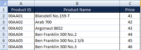
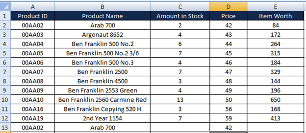
Take this example where we have a list of products. This sheet contains all the products we stock so that in another sheet when we enter a product ID we can draw in the Product Name and Price automatically.

If these are the only products we will ever stock, or if the catalogue only grows very occasionally, then that is ok. We can edit the sheets and formulas as and when required. But what if we are adding new products often?

Thankfully there is a smart way that we can still use VLOOKUP but with a dynamic range. How do we do that? Read on …

VLOOKUP with Named Ranges

Ordinarily when you use VLOOKUP we specify a precise range, such as =VLOOKUP(A2,A2:C10,3) where the range is from A2 to C10. Obviously if we were to add a new product we would need to make it C11 and so on, every time our product list changed.

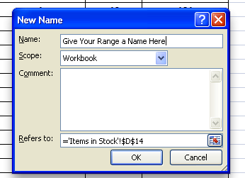
The first step in simplifying this is to instead use a “named range”. So rather than A2:C10 we would use the name “product”.

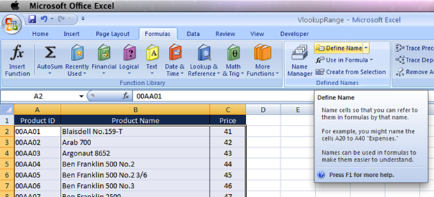
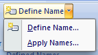
Select the area of cells that you wish to name and click Define Name in the Name Manager.

Then supply the name you wish to use, checking that the range is correct.

This approach now transforms our VLOOKUP to look like VLOOKUP(A2,Product,3) etc. Changing the range then would be simply done centrally in the Name Manager.

Dynamic Named Ranges

We don’t want to have to keep going into Name Manager though. Ideally we want it to “self correct” and just work. The good news is a solution does exist.

When we create the named range, instead of a straight forward range, instead we use a formula.

=OFFSET('Product List'!$A$1,1,0,COUNTA('Product List'!$A:$A)-1,3)

The OFFSET function asks for a row count, but we can even dynamically supply this by using the COUNTA function. Any time we add products this count will increase, giving us our dynamic range.

Summary

A standard VLOOKUP is a great way to speed up your data entry but requires you to edit your formulas or at least the named ranges. Making your named ranges dynamic by using a formula to select the range allows you to focus purely on the data entry, leaving Excel to worry about where your lookups are pointing.

P.S.

Don’t forget to check out our PDF To Excel Converter. It can save you a lot of precious time and improve your productivity.