A Creative Way to Create Re-Usable Macros in Record Time

Microsoft Excel makes it easy to sort a simple table of data. It is a standard operation that most Excel users will visit often. What, though, if you want to perform the sort as part of a macro?

We know that anything a user can do we can normally do within a macro script, the ability to perform a sort is a given … but how can we make a general purpose sorting macro so we can use it in any Excel spreadsheet?

There is little point reinventing the wheel over and over. After all, macros are there to stop us doing repetitive tasks manually. Let us take a look how we can take a macro and make it generic enough that it becomes reusable, and therefore far more useful!

Recording a Macro

First we can start by recording the sorting macro to see how that works. Excel allows us to “record” us performing an operation then “play back” the steps. What it actually does which is pretty smart is puts the steps together in programming code, so we can use it as the foundation for our macro script.

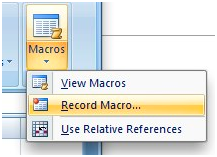
To start the macro recording, find the “Record Macro” command from the “Macros” sub-menu of the “View” bar (I named my macro ‘Sorting’. Go figure).

Next, initiate the sort operation using the “Sort” command from the Data bar, selecting the “Atomic Number” column from the columns combo box in the Sort dialog.

Hit “OK”, and the sorting is done. You can then end the recording using the Stop Recording option from the Macro sub-menu.

As mentioned earlier, behind the scenes you were just generating code. Let’s see what we’ve got here:

As you can see, each macro in Excel is generated as a Sub. My one shown is called “Sorting”.

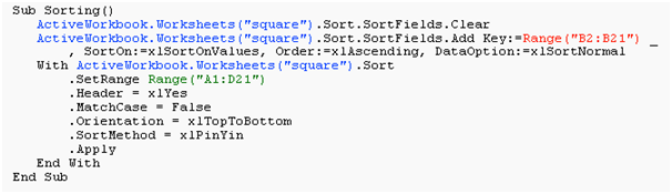
The first three rows in the actual macro clear the old sort (if any), and add new one based on the second column (B). Then the sort options are set, including the range on which to perform the sort, and the existence of a header on the range.

Finally, the sort is applied using the chosen parameters.

Making the Macro More Useful

So far it would be just as easy to run your sort from the standard Excel menu system. Let’s make it more customized.

In order to easily run the macro without having to use the “View Macro” command and then press the “Run” button, I used the “Options” button on the View Macro page and set a keyboard shortcut to the Sorting macro – specifically, Ctrl+Shift+S. When the file is open, you can use that keyboard shortcut to run the macro, sorting the table as quick as a flash.

OK, now we are getting somewhere. It’s a great macro, and I can use it any time to sort any sheet, except for a few problems:

1. It will only work on a worksheet called “square”.
2. It will only work on the exact same number of columns and rows.
3. It will only sort according to the B column.

Well, that simply will not do. We are trying to make life easier, rather than force our spreadsheet to match our macro! So we need to generalize the macro to overcome those problems and make it a “one size fits all” solution.

Here is what we need to do:

1. Use the current worksheet.
2. Get the used range from the sheet so the sorting will affect all columns.
3. Use the currently selected cell’s column as the key for the sorting.

Using the Current Worksheet

Excel macros have a shortcut name for the current worksheet called “ActiveSheet”. Wherever it appears in a macro, Excel will use the currently active worksheet. This will make it easy to fix the first issue, seeing as the recorded macro only applies to the specific sheet it was recorded on.

Next, for simplicity sake assuming we would like to sort all the data in the sheet, we need to find out the last column and row in the sheet that has data in it.

To do this, we can use a neat property called “UsedRange”. When using the property in a macro, Excel replaces it with a square block of cells containing all rows and columns from the first used cell to the last.

So, to sort the whole data in the sheet, regardless of the actual size and shape of it, we can set the sort’s range to work on the whole used range:

.SetRange ActiveSheet.UsedRange

Finally, we really need to be able to sort the table according to any column rather than hard-code it to perform the sort using the same column each time. To make it easier to code, I decided to use the currently selected cell. To do this, we need a few things:

1. Find the selected cell.
2. Get the column from the selected cell.
3. Find the last used row.

From those pieces of info, we can build the key’s range definition.

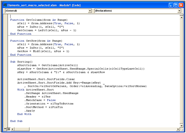
Lucky for you I have created two functions that will return the column and the row of a cell I pass to them called, funnily enough, “Get Column” and “Get Row” (you can see them at the end of the article).

Basically we get the address of the cell as column$row (for example, “B$12″), and then keep the part before the $ sign to get the column, and after to get the row.

The selected cell can be accessed by a macro using “ActiveCell”, much the same as the active worksheet can be accessed via “ActiveSheet”. To get the last cell of the used range, I used a range property that returns the last cell in the range; SpecialCells(xlCellTypeLastCell). Using it on the UsedRange of the sheet returns the last used cell, from which I took the row.

Now we have all the necessary data to create the sort key range. We’ll replace the original “B2:B21″ with “2:“:

sKey = sSortColumn & "2:" & sSortColumn & sLastRow

And then use this to create the key.

ActiveSheet.Sort.SortFields.Add Key:=Range(sKey) _
 , SortOn:=xlSortOnValues, Order:=xlAscending, DataOption:=xlSortNormal

The full macro now looks like this:

Now, I can sort the table by any column just by selecting any cell in it and pressing Ctrl+Shift+S and my work here is done!

You can get the file with the whole macro (and assisting functions) here.

P.S.

Don’t forget to check out our PDF to Excel Converter. It can save you a lot of precious time and improve your productivity.