A Colorful Way to Categorize Your Data

One of my husband’s challenges as “manager of the household budget and head of the household purchasing committee” is to work out which purchases were justified and which should be cut down on (or argued over, whatever).

While I am a total computer addict, my husband feels he has better things to do than to spend hours in a spreadsheet working these things out. Also, if I leave it to him, he is going to say all his expenses were completely justified (how many burgers does one man need a day?), and mine are all up for discussion (I am not a shoe-purchasing addict, honest!).

Here is a geeky Microsoft Excel trick that makes adding up your unnecessary expenses quick and easy. Rather than label or categorize your expenses, we can quickly run through our spreadsheet marking these expenses visually, giving both a nice clue at a glance how far off the rails our spending has gone, but also allowing us to add up these expenses with a couple of key presses!

Our Magic Color-Coded Household Budget Spreadsheet

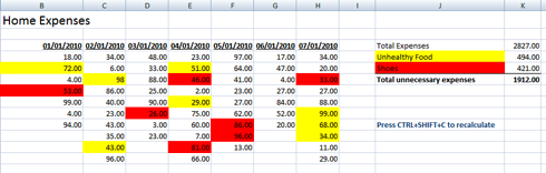
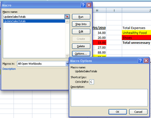
What we decided to do is allocate a color for fast-food purchases, and another color for shoes and other apparel. Then we assign a macro to a keyboard combination which works out the totals to see who wins spent over budget.

Here is how an example spreadsheet might look (no, I am not showing my actual expenses, ha):

Download the example spreadsheet

Yes, yes, I know, his need for burgers ever-so slightly outweighs my shoe purchases. Perhaps he needs to hack in a fail safe …

Building the Cell Color Counting Macro

Anyway, the magic is in the macro, and here it is:

First we create a little subroutine that takes our range of data and finds first the yellow (junk food), and then the red (shoes). We could make the whole thing more generic by making the range flexible but for sake of discussion it is fixed at B4:H13 right now. If you wanted more colours, just duplicate one of the lines and change the target range (eg. To K6), and the colour value (eg. To vbGreen).

Sub UpdateSalesTotals()
    Range("K4").Value = SumInColor(Range("B4:H13"), vbYellow)
    Range("K5").Value = SumInColor(Range("B4:H13"), vbRed)
End Sub

Next is where the real work is done, the SumInColor custom function.

Function SumInColor(rngNumbers As Range, lngColor As Long) As Long
    Dim clSpecificCell As Range
    Dim lngTotal As Long
    lngTotal = 0
    For Each clSpecificCell In rngNumbers
        If clSpecificCell.Interior.Color = lngColor Then _
            lngTotal = lngTotal + clSpecificCell.Value
    Next
    SumInColor = lngTotal
End Function

First we define our variables, then we perform a loop that goes through the supplied range (rngNumbers) looking for the supplied color (lngColor). If it finds the specified color then it adds the found figure to the running total.

Unfortunately, Excel does not seem to have any way we can run this macro automatically when we color a cell, so instead we must use the Options button to set a keyboard shortcut of Ctrl+Shift+C.

Magic isn’t it?

P.S.

Don’t forget to check out our PDF To Excel Converter. It can save you a lot of precious time you now spend on retyping PDF data.